Fourier Series
What do we want to do?
We want to find a polynomial function that can plot any kind of 2D shape using only sampled points. We will use Fourier series to solve this problem.
First, lets sample some points from an image
To sample points, we will use svg files and sample points from the path elements.
1. Parse svg file
An svg file is composed of paths, each paths is composed of segment, a segment can be a line or a curve (eg. CubicBezier).
from svgpathtools import svg2paths
from IPython.display import SVG

paths = svg2paths('formula.svg')[0]

print(f'''number of paths: {len(paths)}
number of elements in `paths[0]`: {len(paths[0])}
type of `paths[0][0]`: {type(paths[0][0])}''')

SVG('formula.svg')
number of paths: 30
number of elements in `paths[0]`: 53
type of `paths[0][0]`: <class 'svgpathtools.path.CubicBezier'>

Moreover, the svgpathtools library give us the access to the polynomial function that describe each segment. Each segment polynome takes a parameter in and return a complex number. The complex number is the point on the segment for the given parameter .
Here for example, we sampled 20 points from the 35th segment of the 2nd path:
t = np.linspace(0, 1, 20)
segment = paths[2][35]

scatter(segment.poly()(t));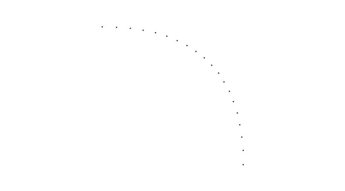
2. Sample points from svg file
Our goal here is to sample points from the svg file. By using the length each segments, we can sample the points proportionally to the length of each segment.
N_POINTS = 1000

total_length = sum(path.length() for path in paths)

def get_t(seg):
  prop = seg.length() / total_length
  n = round(prop * N_POINTS)
  if n == 1:
    return [.5] # center of the segment
  return np.linspace(0, 1, n)

sampled_points_by_path = []
for path in paths:
  path_points = [seg.poly()(get_t(seg)) for seg in path]
  path_points = np.hstack(path_points)
  sampled_points_by_path.append(path_points)

scatter(sampled_points_by_path[6],
        title='Sampled points of the 6th path');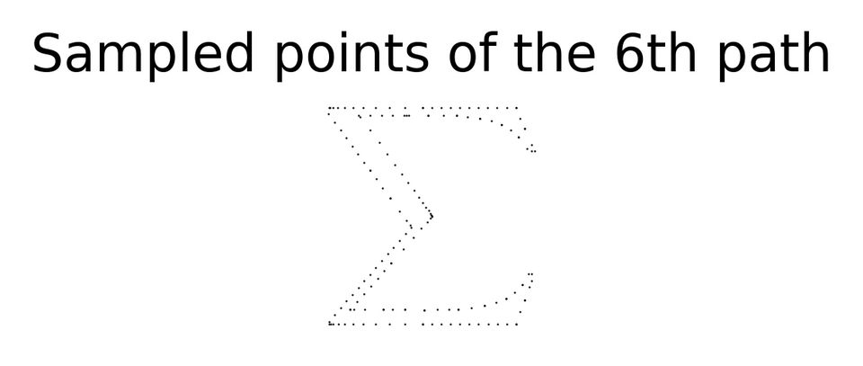
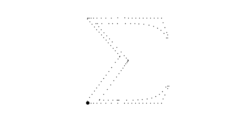
The sampled points of the image looks like this:
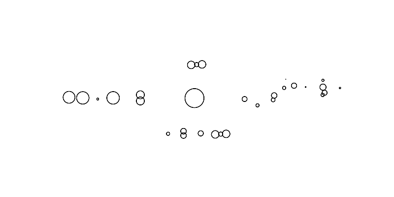
scatter(sampled_points_by_path,
        title=f'Sampled points');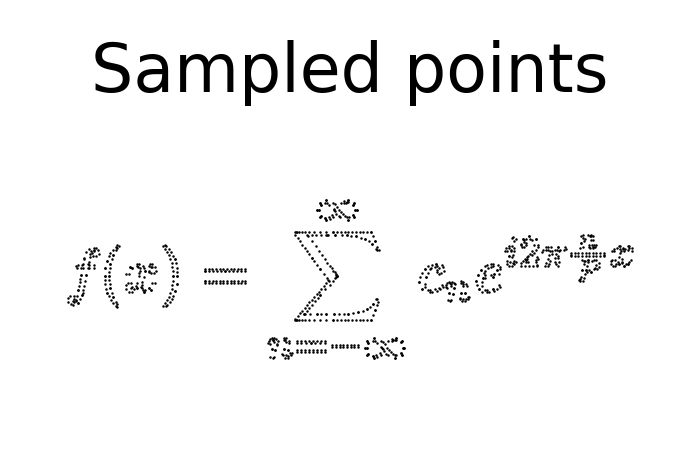
Using the sampled points, we can now create the reference function
The idea is to create a reference function for each path that maps the time to the closest sampled point to the time of the path .
def f_data_i(i, t):
  points = sampled_points_by_path[i]
  closest_idx = (t*(points.shape[0]-1)).astype(int)
  return points[closest_idx]

def f_data(t):
  return [f_data_i(i, t)
          for i in range(len(sampled_points_by_path))]
For example, bellow, the big circle is the plot of which plots the 6th path with going from to .
Of course, we could use these points to plot the final image but the resulted function will not be smooth nor a polynome.
For brievity, we will use the notation for the rest of the notebook that refers to one of the reference functions .
Now, we can use the to compute the Fourier coefficients
Recap that, here, the Fourier series of is given by
To extract the coefficients , we multiply both sides by and integrate over the interval :
def compute_c_i(i, n):
  t = np.linspace(0, 1, 1000)
  fx = f_data_i(i, t)
  integrand = fx*np.exp(-2j*np.pi*n[:, None]*t)
  cn = np.trapz(integrand)
  return cn
We can now approximate the reference function with a truncated Fourier series.
def f_approx_i(i, t, n_freqs):
  n = np.arange(-n_freqs//2, n_freqs//2+1)
  cn = compute_c_i(i, n)
  n, cn = n[:, None], cn[:, None] # add new axis for broadcasting
  f_approx = np.sum(cn*np.exp(2j*np.pi*n*t), axis=0)
  return f_approx

def f_approx(t, n_freqs):
  return [f_approx_i(i, t, n_freqs)
          for i in range(len(sampled_points_by_path))]

t = np.linspace(0, 1, 1000)
plot(f_approx(t, n_freqs=6),
     title=f'Fourier approximation (#freqs=5)');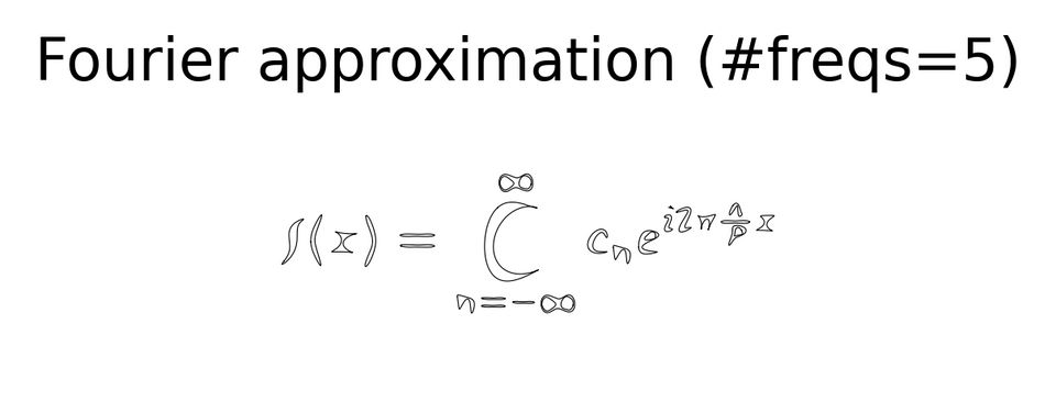
Here, for example, the number "2" symbole (22th path) can be represented by the following polynomials:
cn = np.array([
  -438-104j,
  40-60j,
  354-1141j,
  156814+19842j,
  -1200-1724j,
  62+39j,
  -121+657j])

t = np.linspace(0, 1, 1000)
n = np.arange(-3, 4)
cn, n = cn[:,None], n[:,None]
f_22 = np.sum(cn * np.exp(2j * np.pi * n * t), axis=0)

plot(f_22, title='Approximation of $f_{data}^{(22)}$');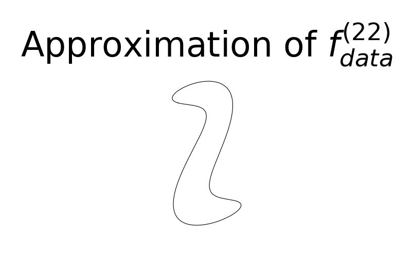
We're done, we can play with the number of frequencies to get accurate result